{All Code} {Session Info} {Updates}
I recently posted a GIF of our new transcriptomics clustering in the form of a tSNE plot, which appears to resolve from a cloud of random points into a nice, orderly structure. Below, I’ll show how this was built with the help of gganimate, tweenr, and of course ggplot2 in R.
Fun with gganimate and tweenr while I wait for our ms to get through @biorxivpreprint screening. #rstats #gganimate #tsne pic.twitter.com/5OvRuQGbhw
— Lucas Graybuck (@hypercompetent) December 7, 2017
The main gist of the process is that we need to set up several states for the points to shift between, which the tweenr package will interpolate to generate all of the positions in each frame, and then the gganimate package (along with ImageMagick if you’d like to make a GIF) can be used to build an animation.
To get started, you’ll need to download gganimate and tweenr from Github using the devtools package:
if (!require(devtools)) {
    install.packages("devtools")
}
if (!require(gganimate)) {
  devtools::install_github("dgrtwo/gganimate")
}
if (!require(tweenr)) {
  devtools::install_github("thomasp85/tweenr")
}
In addition to these packages, I’ll also use dplyr for data manipulation, ggplot2 for plotting, and data.table to quickly read the data from .csv.
library(data.table)
library(dplyr)
library(ggplot2)
library(gganimate)
library(tweenr)
In this demo, I’ll be starting with tSNE coordinates and cluster labels for each point that we’ve generated previously. These can be retrieved from Github:
tsne_dims <- fread("https://github.com/hypercompetent/plottery_barn_data/raw/master/gganimate-tweenr-tsne-plot/tsne_dims.csv")

head(tsne_dims)
## sample_id cluster_id cluster_color tsne_x tsne_y
## 1: LS-14690_S02_E1-50 35 #994C00 25.07267 -2.7706899
## 2: LS-14690_S03_E1-50 56 #00979D -39.18723 20.9199491
## 3: LS-14690_S05_E1-50 56 #00979D -44.35434 12.0985906
## 4: LS-14690_S06_E1-50 56 #00979D -42.82413 21.0532487
## 5: LS-14690_S07_E1-50 56 #00979D -42.08457 0.6795734
## 6: LS-14690_S08_E1-50 56 #00979D -41.15694 13.0337231ggplot() +
geom_point(data = tsne_dims,
aes(x = tsne_x,
y = tsne_y,
color = cluster_color)) +
scale_color_identity() +
theme_void()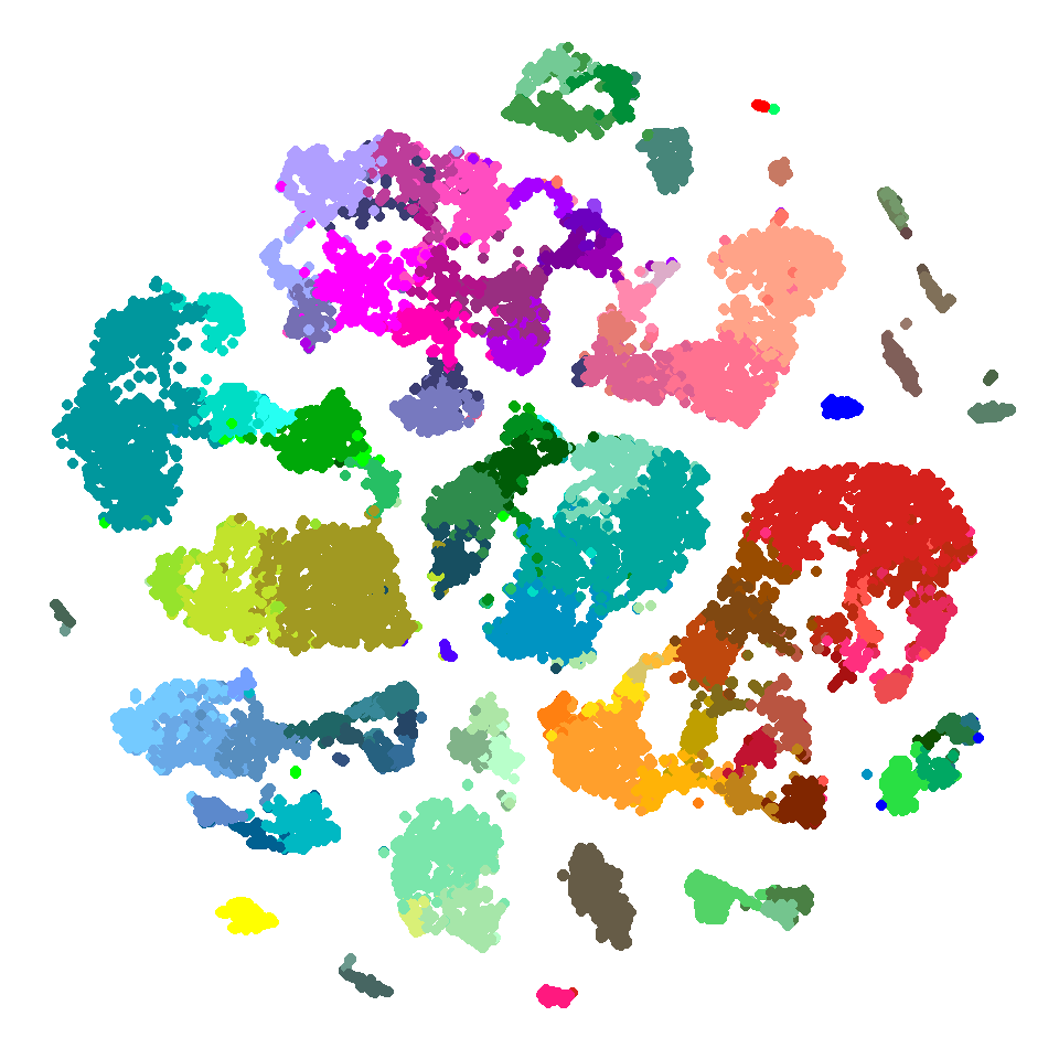
At the beginning of the animation, I’d like all of the points to start in a random position, and come into focus in their tSNE positions. This function will generate random positions for num_points distributed over the surface of a disc with the given disc_radius.
random_disc_jitter <- function(num_points,
disc_radius,
random_seed = 42) {
if(!is.null(random_seed)) {
set.seed(random_seed)
}
# Random radius positions
r <- runif(num_points, 0, disc_radius ^ 2)
# Random angles
t <- runif(num_points, 0, 2 * pi)
# Convert radius and angles to cartesian coordinates
data.frame(x = sqrt(r) * cos(t),
y = sqrt(r) * sin(t))
}I’ll use dplyr’s mutate() to add this to the tsne_dims data:
# Get the max x or y value from the tsne dims.
# I'll use this for the radius
max_tsne <- max(abs(c(tsne_dims$tsne_x, tsne_dims$tsne_y)))
tsne_dims <- tsne_dims %>%
mutate(random_x = random_disc_jitter(num_points = n(),
disc_radius = max_tsne)$x,
random_y = random_disc_jitter(num_points = n(),
disc_radius = max_tsne)$y)
head(tsne_dims)## sample_id cluster_id cluster_color tsne_x tsne_y
## 1 LS-14690_S02_E1-50 35 #994C00 25.07267 -2.7706899
## 2 LS-14690_S03_E1-50 56 #00979D -39.18723 20.9199491
## 3 LS-14690_S05_E1-50 56 #00979D -44.35434 12.0985906
## 4 LS-14690_S06_E1-50 56 #00979D -42.82413 21.0532487
## 5 LS-14690_S07_E1-50 56 #00979D -42.08457 0.6795734
## 6 LS-14690_S08_E1-50 56 #00979D -41.15694 13.0337231
## random_x random_y
## 1 52.58733 10.462040
## 2 -54.22300 -2.175301
## 3 -24.48068 17.318257
## 4 32.24114 39.626810
## 5 -16.53971 -41.751597
## 6 31.92132 24.745645ggplot() +
geom_point(data = tsne_dims,
aes(x = random_x,
y = random_y,
color = cluster_color)) +
scale_color_identity() +
theme_void()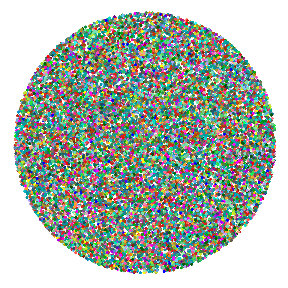
For the final state in the animation, I’d like the points to gather around their cluster centroids. A nice way to densely pack points is with Fermat’s spiral. Thanks to a StackOverflow reply by user Manish Nag, I was able to write a function to arrange points along this spiral.
This function will generate coordinates for num_points around a central position (center_x and center_y), and return x and y coordinates for spiral positioning in a circle with radius supplied by the size argument. I’ll use this to generate positions for the third phase of the plot, which gathers the points around the centroid for each cluster.
fermat_jitter <- function(num_points,
size,
center_x,
center_y) {
golden_ratio <- (sqrt(5) + 1) / 2
fibonacci_angle <- 360 / (golden_ratio ^ 2)
ci <- sqrt(size / num_points)
x <- rep(center_x, num_points)
y <- rep(center_y, num_points)
for (m in 1:(num_points - 1)) {
n <- m - 1
r <- ci * sqrt(n)
theta <- fibonacci_angle * (n)
x[n] <- center_x + r * cos(theta)
y[n] <- center_y + r * sin(theta)
}
data.frame(x = x,
y = y)
}To generate these for the plot, I’ll use dplyr’s group_by() function to find the centroid of each cluster in tSNE coordinates, then jitter around the centroids using the fermat_jitter() function.
# Some trial and error for this value to find a size that packs the points without getting
# too much overlap
max_size <- 16
# We'll also need the max cluster n to scale the jitter radius
max_n <- max(table(tsne_dims$cluster_id))
tsne_dims <- tsne_dims %>%
group_by(cluster_id) %>%
mutate(centroid_x = mean(tsne_x, trim = 0.5),
centroid_y = mean(tsne_y, trim = 0.5)) %>%
mutate(fermat_x = fermat_jitter(num_points = n(),
size = max_size * n() / max_n,
center_x = centroid_x[1],
center_y = centroid_y[1])$x,
fermat_y = fermat_jitter(num_points = n(),
size = max_size * n() / max_n,
center_x = centroid_x[1],
center_y = centroid_y[1])$y) %>%
ungroup()
head(tsne_dims)## # A tibble: 6 x 11
## sampl~ clust~ clus~ tsne~ tsne_y rand~ rando~ cent~ centr~ ferm~ ferma~
## <chr> <int> <chr> <dbl> <dbl> <dbl> <dbl> <dbl> <dbl> <dbl> <dbl>
## 1 LS-14~ 35 #994~ 25.1 - 2.77 52.6 10.5 25.5 - 4.84 25.6 - 4.91
## 2 LS-14~ 56 #009~ -39.2 20.9 -54.2 - 2.18 -42.7 12.4 -42.6 12.3
## 3 LS-14~ 56 #009~ -44.4 12.1 -24.5 17.3 -42.7 12.4 -42.7 12.2
## 4 LS-14~ 56 #009~ -42.8 21.1 32.2 39.6 -42.7 12.4 -42.8 12.2
## 5 LS-14~ 56 #009~ -42.1 0.680 -16.5 -41.8 -42.7 12.4 -42.9 12.3
## 6 LS-14~ 56 #009~ -41.2 13.0 31.9 24.7 -42.7 12.4 -42.9 12.5ggplot() +
geom_point(data = tsne_dims,
aes(x = fermat_x,
y = fermat_y,
color = cluster_color)) +
scale_color_identity() +
theme_void()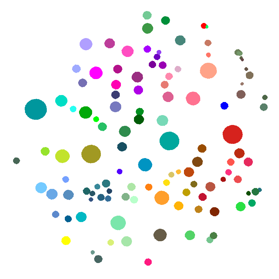
For gganimate and tweenr, I’ll need these to be separate data frames with matching column names.
state_1 <- data.frame(x = tsne_dims$random_x,
y = tsne_dims$random_y,
color = tsne_dims$cluster_color)
state_2 <- data.frame(x = tsne_dims$tsne_x,
y = tsne_dims$tsne_y,
color = tsne_dims$cluster_color)
state_3 <- data.frame(x = tsne_dims$fermat_x,
y = tsne_dims$fermat_y,
color = tsne_dims$cluster_color)Now, tweenr can be used for interpolation. To get a round-trip animation, I’ll build a list of states that goes from 1 -> 2 -> 3 -> 2 -> 1. The “cubic-in-out” option for the ease parameter applies some acceleration to the points at the beginning and end of each transition, which makes it look smoother.
state_list <- list(state_1, state_2, state_3, state_2, state_1)
tweened_states <- tween_states(state_list,
tweenlength = 2,
statelength = 1,
ease = "cubic-in-out",
nframes = 96)Then, the plot can be assembled with the frame aesthetic, which will be used by gganimate to build the animation.
tweened_plot <- ggplot(data = tweened_states,
aes(x = x,
y = y)) +
geom_point(aes(frame = .frame,
color = color),
size = 1.5) +
scale_color_identity() +
theme_void()## Warning: Ignoring unknown aesthetics: frameFinally, gganimate can be used to build a GIF of the animation.
Side note: In order to get GIF output (at least on Windows, which is where I’m using this), you’ll need ImageMagick. The easiest way I’ve found to get this to work is to get the portable version of ImageMagick. I installed this at C:/ImageMagick/, which I need to add to the R PATH to get gganimate to work.
Sys.setenv(PATH = paste("C:/ImageMagick/",
Sys.getenv("PATH"),
sep = ";"))
gganimate(tweened_plot,
"tsne_to_centroids_twitter.gif",
ani.width = 506,
ani.height = 506,
interval = 1/8,
title_frame = F)
And that’s it! Note that the plot can be made smoother and clearer by making a larger version (increase nframes in tween_states(), and increase ani.width and ani.height in gganimate()) at the expense of more time to generate the additional frames, and a larger final file size.
All Code
Below is all of the code together in one section.
library(dplyr)
library(ggplot2)
library(gganimate)
library(tweenr)
library(data.table)
## tSNE dimensions
tsne_dims <- fread("https://github.com/hypercompetent/plottery_barn_data/raw/master/gganimate-tweenr-tsne-plot/tsne_dims.csv")
head(tsne_dims)
ggplot() +
  geom_point(data = tsne_dims,
             aes(x = tsne_x,
                 y = tsne_y,
                 color = cluster_color)) +
  scale_color_identity() +
  theme_void()
## Random dimensions
random_disc_jitter <- function(num_points,
                               disc_radius,
                               random_seed = 42) {

  if(!is.null(random_seed)) {
    set.seed(random_seed)
  }

  # Random radius positions
  r <- runif(num_points, 0, disc_radius ^ 2)
  # Random angles
  t <- runif(num_points, 0, 2 * pi)

  # Convert radius and angles to cartesian coordinates
  data.frame(x = sqrt(r) * cos(t),
             y = sqrt(r) * sin(t))
}
# Get the max x or y value from the tsne dims.
# I'll use this for the radius
max_tsne <- max(abs(c(tsne_dims$tsne_x, tsne_dims$tsne_y)))

tsne_dims <- tsne_dims %>%
  mutate(random_x = random_disc_jitter(num_points = n(),
                                       disc_radius = max_tsne)$x,
         random_y = random_disc_jitter(num_points = n(),
                                       disc_radius = max_tsne)$y)

head(tsne_dims)
ggplot() +
  geom_point(data = tsne_dims,
             aes(x = random_x,
                 y = random_y,
                 color = cluster_color)) +
  scale_color_identity() +
  theme_void()
## Fermat spiral dimensions
fermat_jitter <- function(num_points,
size,
center_x,
center_y) {
golden_ratio <- (sqrt(5) + 1) / 2
fibonacci_angle <- 360 / (golden_ratio ^ 2)
circle_r <- sqrt(size / num_points)
x <- rep(center_x, num_points)
y <- rep(center_y, num_points)
for (m in 1:(num_points - 1)) {
n <- m - 1
r <- circle_r * sqrt(n)
theta <- fibonacci_angle * (n)
x[n] <- center_x + r * cos(theta)
y[n] <- center_y + r * sin(theta)
}
data.frame(x = x,
y = y)
}
# Some trial and error for this value to find a size that packs the points without getting
# too much overlap
max_size <- 16
# We'll also need the max cluster n to scale the jitter radius
max_n <- max(table(tsne_dims$cluster_id))

tsne_dims <- tsne_dims %>%
  group_by(cluster_id) %>%
  mutate(centroid_x = mean(tsne_x, trim = 0.5),
         centroid_y = mean(tsne_y, trim = 0.5)) %>%
  mutate(fermat_x = fermat_jitter(num_points = n(),
                                  size = max_size * n() / max_n,
                                  center_x = centroid_x[1],
                                  center_y = centroid_y[1])$x,
         fermat_y = fermat_jitter(num_points = n(),
                                  size = max_size * n() / max_n,
                                  center_x = centroid_x[1],
                                  center_y = centroid_y[1])$y) %>%
  ungroup()

head(tsne_dims)
ggplot() +
  geom_point(data = tsne_dims,
             aes(x = fermat_x,
                 y = fermat_y,
                 color = cluster_color)) +
  scale_color_identity() +
  theme_void()
## Build the animation
state_1 <- data.frame(x = tsne_dims$random_x,
                      y = tsne_dims$random_y,
                      color = tsne_dims$cluster_color)

state_2 <- data.frame(x = tsne_dims$tsne_x,
                      y = tsne_dims$tsne_y,
                      color = tsne_dims$cluster_color)

state_3 <- data.frame(x = tsne_dims$fermat_x,
                      y = tsne_dims$fermat_y,
                      color = tsne_dims$cluster_color)
state_list <- list(state_1, state_2, state_3, state_2, state_1)

tweened_states <- tween_states(state_list,
                               tweenlength = 2,
                               statelength = 1,
                               ease = "cubic-in-out",
                               nframes = 96)
tweened_plot <- ggplot(data = tweened_states,
aes(x = x,
y = y)) +
geom_point(aes(frame = .frame,
color = color),
size = 1) +
scale_color_identity() +
theme_void()
# May need to set the path
#Sys.setenv(PATH = paste("C:/ImageMagick/",
# Sys.getenv("PATH"),
# sep = ";"))
gganimate(tweened_plot,
"tsne_to_centroids.gif",
ani.width = 300,
ani.height = 300,
interval = 1/8,
title_frame = F)Session Info
sessionInfo()## R version 3.4.3 (2017-11-30)
## Platform: x86_64-w64-mingw32/x64 (64-bit)
## Running under: Windows 10 x64 (build 16299)
##
## Matrix products: default
##
## locale:
## [1] LC_COLLATE=English_United States.1252
## [2] LC_CTYPE=English_United States.1252
## [3] LC_MONETARY=English_United States.1252
## [4] LC_NUMERIC=C
## [5] LC_TIME=English_United States.1252
##
## attached base packages:
## [1] methods stats graphics grDevices utils datasets base
##
## other attached packages:
## [1] bindrcpp_0.2 tweenr_0.1.5.9999 gganimate_0.1.0.9000
## [4] ggplot2_2.2.1 dplyr_0.7.4 data.table_1.10.4-3
##
## loaded via a namespace (and not attached):
## [1] Rcpp_0.12.14 pillar_1.0.1 compiler_3.4.3 plyr_1.8.4
## [5] bindr_0.1 tools_3.4.3 digest_0.6.13 evaluate_0.10.1
## [9] tibble_1.4.1 gtable_0.2.0 pkgconfig_2.0.1 rlang_0.1.6
## [13] cli_1.0.0 curl_3.1 yaml_2.1.16 blogdown_0.4
## [17] stringr_1.2.0 knitr_1.18 rprojroot_1.3-1 grid_3.4.3
## [21] glue_1.2.0 R6_2.2.2 rmarkdown_1.8 bookdown_0.5
## [25] magrittr_1.5 backports_1.1.2 scales_0.5.0 htmltools_0.3.6
## [29] assertthat_0.2.0 colorspace_1.3-2 labeling_0.3 utf8_1.1.2
## [33] stringi_1.1.6 lazyeval_0.2.1 munsell_0.4.3 crayon_1.3.4Updates
2017-01-07: Added section links to the top of the page.
2017-12-31: First version